


Садржај
Формулисање проблема
It is necessary to make sure that in one of the cells of the sheet there is a drop-down list with names, when selected from which, the product would be displayed next to it as a photo:
видео
Step 1. Create a directory with a photo and give it a name
We create on Листе 1 we are a catalog with names and photos of goods, consisting of two columns (модел и слика):
Now we need to give a name to our directory in order to refer to it in the future. In Excel 2003 and older, for this we go to the menu Insert – Name – Assign (Insert – Name – Define), and in Excel 2007 and newer – click on the button Наме Манагер табулатор формула. Create a range – enter a name (for example фото албум) and specify the formula as the address:
=СМЕЩ(Лист1!$A$1;1;0;СЧЁТЗ(Лист1!$A:$A)-1;1)
=OFFSET(Лист1!$A$1;1;0;COUNTA(Лист1!$A:$A)-1;1)

This formula determines the last occupied cell in column A and outputs the range from A2 to this found cell. Such a relatively complex construction is needed in order to subsequently add new models to our list and not think about correcting the range. If you don’t have to add anything for sure, then instead of entering this scary formula, just enter =A2:A5
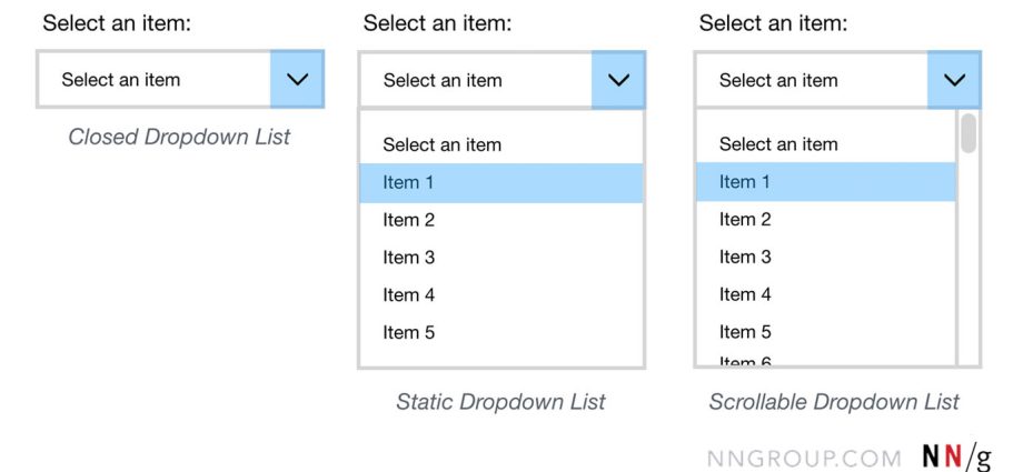
Step 2. Drop-down list for choosing a model
Идемо у Лист КСНУМКС and create a cell there with a drop-down list for the user to select a phone model (let it be A1). Select a cell and go to the menu Подаци – Провера (Подаци – Валидација) or in new versions of Excel – on the tab Data – Data Validation (Data – Data Validation). Further into the field Тип података (Дозволи) Изаберите Листа, већ као извор indicate our фото албум (don’t forget to add an equal sign in front of it):

In addition, it is convenient to give this cell a name – menu again Убаци – Име – Додели and then enter a name (for example Избор) и OK.
Step 3: Copy the Photo
Let’s move the first photo from the photo album to the drop-down list. Select the cell with the first photo (not the picture itself, but the cell!) and
in Excel 2003 and later, hold down Shift to open the menu едит. A previously invisible item should appear there. Copy as Picture:
In Excel 2007 and newer, you can simply expand the dropdown below the button Copy (Copy) on Početna Картица:
In Excel 2010, another additional window will appear with a choice of the type of image to be created:

In it, you need to select the options “as on the screen” and “raster”.
Copy, go to Лист КСНУМКС to the drop-down list and in any empty cell near it, insert our mini-screenshot of the cell with a photo (menu Edit – Paste or the usual ЦТРЛ + В).
Step 4. Create a dynamic link to the selected photo
Now you need to make a link that will point to the cell with the selected photo. Opening the menu Уметнути – Име – Дефинисати or Наме Манагер табулатор формула and create another named range:

The name of our link, let’s say, will be слика, and the formula
=СМЕЩ(Лист1!$B$2;ПОИСКПОЗ(Выбор;Фотоальбом;0)-1;0;1;1)
=OFFSET(Лист1!$B$2;MATCH(Выбор;Фотоальбом;0)-1;0;1;1)
Technically, a function УТАКМИЦА finds a cell with the desired model in the catalog by name, and the function ОФФСЕТ then gives a link to the cell adjacent to the right of the found name, i.e. cell with a photo of the product.
Step 5. Attaching a photo to a link
It remains to select the copied photo on Листе 2 and enter in the formula bar
=слика
и притисните Ентер
All! 🙂
- Create drop down list in worksheet cells
- Креирање зависних падајућих менија
- Аутоматско генерисање падајућих листа помоћу ПЛЕКС додатака
- Падајућа листа са аутоматским брисањем већ коришћених ставки
- Dropdown list with automatic addition of missing items