


Садржај
Sometimes it can be difficult to quickly and efficiently match the timelines of projects. A graphical representation of project deadlines and milestones will help identify any bottlenecks during planning.
Of course, it is worth considering the use of project management systems. Such a system will show the start and end times of the project tasks against the general background. But such systems are quite expensive! Another solution is to try using the Excel timeline bar chart when planning to see all the conflicts in the project. Collaboration with the team and with third-party specialists will be much easier if the actions of everyone can be seen on the same sheet!
Unfortunately, creating a timeline in Microsoft Excel is not an easy task. I would not recommend building a complex Gantt chart in Excel, but a simple timeline can be created by following our step-by-step instructions:
Корак 1: Припремите податке
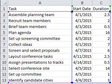
To begin with, we need a data table, in the left column of which (column А) contains all the task names, and the two columns on the right are reserved for the start date and duration of the task (columns В и С).
Корак 2: Направите графикон
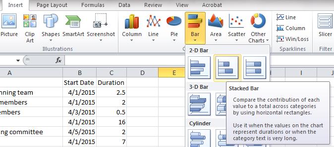
Highlight the prepared data table, then on the tab Убацити (Инсерт) у одељку Дијаграми (Графикони) кликните Рулед Стацкед (Стацкед Бар).
Step 3: Plotting Data on the Chart Correctly
This step is always the most difficult, as the chart is initially plotted with the correct data in the wrong places, if that data ever appeared on the chart!
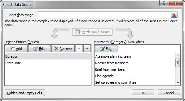
Кликните на дугме Изаберите податке (Изаберите картицу). Конструктор (Design). Check what’s in the area Ставке легенде (редови) (Legend Entries (Series)) two elements are written – duration (Duration) and start date (Start Date). There should be only these two elements.
Let me guess. Has all the information moved or moved to the side? Let’s fix it.
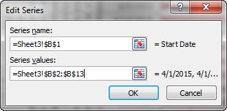
To correct your data, click додати (Додај) или Променити (Edit) in the area Ставке легенде (редови) (Legend Entries (Series)). To add a Start Date, specify a cell B1 на терену Име реда (Series Name), and in the field Вредности (Series Values) – range Б2: Б13. In the same way, you can add or change the duration of tasks (Duration) – in the field Име реда (Series Name) specify a cell C1, and in the field Вредности (Series Values) – range Ц2: Ц13.
To tidy up the categories, click the button Променити (Edit) in the area Ознаке хоризонталне осе (категорије) (Horizontal (Category) Axis Labels). The data range should be specified here:
=Лист3!$A$2:$A$13
=Sheet3!$A$2:$A$13
At this point, the chart should look like a stacked chart with task titles on the vertical axis and dates on the horizontal axis.
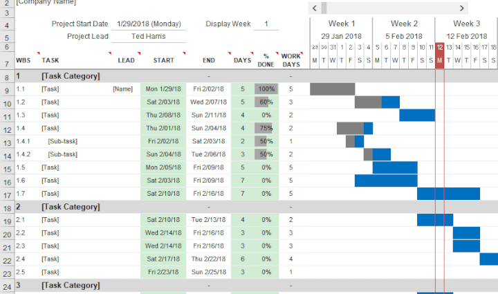
Step 4: Turning the Result into a Gantt Chart
All that remains to be done is to change the fill color of the leftmost parts of all the resulting graph bars to either white or transparent.
★ Read more about creating a Gantt chart in the article: → How to build a Gantt chart in Excel – step by step instructions
Step 5: Improving the Look of the Chart
The final step is to make the diagram prettier so that it can be sent to the manager. Check the horizontal axis: only the project duration bars should be visible, i.e. we need to remove the empty space that appeared in the previous step. Right-click on the horizontal axis of the chart. A panel will appear Параметри осовине (Axis Options), in which you can change the minimum value of the axis. Customize the colors of the Gantt chart bars, set something more interesting. Lastly, don’t forget the title.
Timeline in Excel (Gantt chart) can be used for various purposes. Management will surely appreciate that you can create such a schedule without the extra expense of buying expensive project management software!