


Садржај
- pattern fill
- Save Excel charts as a picture
- Row overlap and side clearance adjustment
- Big Data Series
- Plotting on the Second Axis
- Креирајте комбиноване графиконе
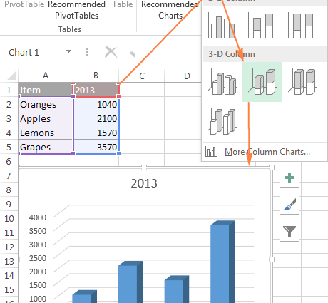
- Automatically create Excel charts
- Smart Chart Titles
- Excel Chart Color Changes
- Managing nulls and missing data
- Plotting Discontiguous Data
- Save a chart as a template
Tips, tricks, and techniques to improve the look of charts in Microsoft Excel.
The charting tools in Microsoft Excel 2010 and 2007 are much better in appearance and functionality than those available in earlier versions of Excel. Although the graphs look better, not all parameters that are used to increase functionality are immediately evident. This short article covers useful tips, tricks and methods for creating charts in Excel that will make your work more efficient.
pattern fill
An update in Microsoft Office 2010 is the ability to use chart pattern fills in grayscale. To see this in action, highlight the diagram, select “Chart Tools” → “Layout tab” and select an edit option from the drop-down list at the top left of the ribbon. Select “Select Format” (just below that on the ribbon) and select “Fill” → “Pattern fill”. For a black and white chart, set the foreground color to black and the background color to white, and select a fill pattern for the series. Repeat steps for another template. You don’t have to use black and white, try different templates to make sure the charts are legible when printed in black and white or copied in black and white.
Templates can be used to fill out a chart in Excel 2010 so that it can be printed in black and white or copied in black and white.
Save Excel charts as a picture
You can save a chart as a picture from Excel for use in other documents such as reports or the web. To save a chart as a picture, the easiest way is to size the chart on the worksheet so that it is large. To perform this operation, you must go along the path: Фајл → Сачувај као, select the path to save the final file and in the drop-down list “Save type” select a web page (*.htm;*.html), enter a name for the new file and click the Save button.
As a result, the worksheet is converted to an html file, and since html files cannot contain images, the chart is saved separately and linked to the html file. The chart will be saved in the folder where the html file was saved to. So if the file was named Sales.htm, then the images would be in a folder called sales_files. The images are saved as a separate PNG file. If the diagram and this Excel file are still needed for work, it must also be saved separately.
The chart can be saved as a graphic file if you later need it for another project.
Row overlap and side clearance adjustment
The appearance of the chart can be improved by changing the width of the rows and the side gaps between them. To adjust the overlap between two series of charts or change the distance between them, right-click on any row on the chart and click „Формат серије података“. Use the Overlap Rows feature to split rows or merge rows by dragging the slider to Gap or Overlap.
Thus, the distance between the rows is adjusted so that they are closer or farther apart. If there are two types of data in the chart, and they need to be superimposed on each other, and the second row should be superimposed on the first, then the order of constructing the chart changes. First, the desired overlap is established. Then right-click to select the data series and select „Изабери податке“. Next, row 1 is selected and moved down to row 2. By changing the order of the tables in this way, smaller data can be displayed in front of larger ones.
Big Data Series
When plotting data based on dates, the data series is often too narrow. The solution to this question is to highlight the x-axis (horizontal axis) of the excel chart, right-click and select the axis format. After choosing the axis options, you need to click on the text axis to select it. In this way, the desired row width can be adjusted. In addition to rows, you can adjust the distance between them.
Plotting on the Second Axis
When plotting small data, such as percentages, that are adjacent to large data, such as millions, the percentages will be lost and not visible. The problem is solved by constructing a percentage chart on a different axis. For this, a diagram is selected and in the tab „Рад са графиконима“, the tab is selected Распоред, which is located in the upper left corner. You want to select rows that are not visible. Then press the button “Format Selection”, which will appear immediately below, then in the group „Опције реда“ одабрати “Secondary Axis” and close the window. Without moving the selected element, select „Рад са графиконима“, then – tab Constructor, а затим изаберите „Промени тип графикона“.
You can now select a different chart type, such as Line. Because a series has been chosen that will apply only to that series and not to the entire chart, the result is a combined chart, such as a bar chart with a line chart on top. A chart looks better and is easier to read if the text on its axis matches the color of the part of the chart that contains the data. Therefore, if there are green rows, it is better to type the corresponding text also in green, and the red row will be displayed in red on its axis.
Креирајте комбиноване графиконе
Microsoft Excel users are not immediately aware that it can create combo charts; however, this is easy to do. To do this, data is selected and the first type of chart is built, for example, a row chart. Then a series is selected that needs to be shown in a different way, for example, using a line chart, and “Working with diagrams” → tab “Constructor” → „Промени тип графикона“ and the second chart type is selected. Some types of charts cannot be combined for reasonable reasons, such as two line charts, but line and line charts work well together.
Automatically create Excel charts
If you have data that will grow over time, you can create a chart so that it grows larger as more data is added to the data warehouse. To do this, the data must be formatted as a table. To do this, already entered data is selected, and on the tab "Почетна" function is selected „Форматирај као табелу“. Now, because the data is formatted as a table, when you create a chart on tabular data, adding more data to the table will automatically expand the chart.
Smart Chart Titles
The title of the chart can be pulled from one of the cells on the Excel sheet. First, a chart title is added in the “Working with diagrams” → Картица Лаиоут → „Наслов графикона“ and is placed, for example, above the diagram. The cell for the title of the chart is selected, then the cursor is moved to the formula bar and a reference is entered to the cell containing the data that will serve as the title of the chart. If the chart title should be the same as the sheet, cell D5 on sheet 1 should be blank. Now, whenever the content of that cell changes, the title of the chart also changes.
Excel Chart Color Changes
For charts with one kind of data, you may notice that Excel colors each series with the same color. This can be changed by clicking on the row and right-clicking on it, after which you will need to select the tab “Format Data Series”, и онда - “Пуњење”. If the chart displays only one data series, you can select the option “Colorful Dots”.
Of course, you can always select an individual data series, right-click and select “Data Point Format”and then set any color for that data point.
Managing nulls and missing data
When there are zero values or missing data in the chart, you can control the display of zeros by selecting the chart row, then − „Рад са графиконима“ → tab “Constructor” → „Изабери податке“ → “Hidden and empty cells”. Here you can choose whether empty cells are displayed as spaces or zero, or if the chart is a line chart, whether the line should run from point to point instead of a blank value. After selecting the required data, the settings are saved by pressing the button "У РЕДУ".
Нотес. This only applies to missing values, not nulls.
Plotting Discontiguous Data
To plot data that is not lined up as side by side series, hold down the Ctrl key after first selecting the data for each range. After you select a range, a chart is created based on the selected data.
Save a chart as a template
To save a chart as a template so that it can be used again, you first create and customize the desired look of the chart. Select the chart, click „Рад са графиконима“, then the tab opens „Конструктор” and the button is pressed “Save as Template”. You will need to enter a name for the chart and click саве. This format can then be applied to other diagrams using the saved template when creating a new diagram or editing an existing one. To apply the saved template, you need to select the chart. To select it, follow the chain: “Working with charts”→ “Constructor → Промените тип графикона → Dezeni. Then select the previously created template and click the “OK” button.
These charting tips and tricks help you create beautiful charts faster and more efficiently in Excel 2007 and 2010.