


Садржај
In the second part of our tutorial on the function ВПР (VLOOKUP) in Excel, we will analyze a few examples that will help you direct all the power ВПР to solve the most ambitious Excel tasks. The examples assume that you already have a basic knowledge of how this feature works. If not, you might be interested in starting with the first part of this tutorial, which explains the syntax and basic usage. ВПР. Па, хајде да почнемо.
Search in Excel by multiple criteria
функција ВПР in Excel is a really powerful tool for performing searches for a particular value in a database. However, there is a significant limitation – its syntax allows you to search for only one value. What if you want to search by multiple conditions? You will find the solution below.
Example 1: Search by 2 different criteria
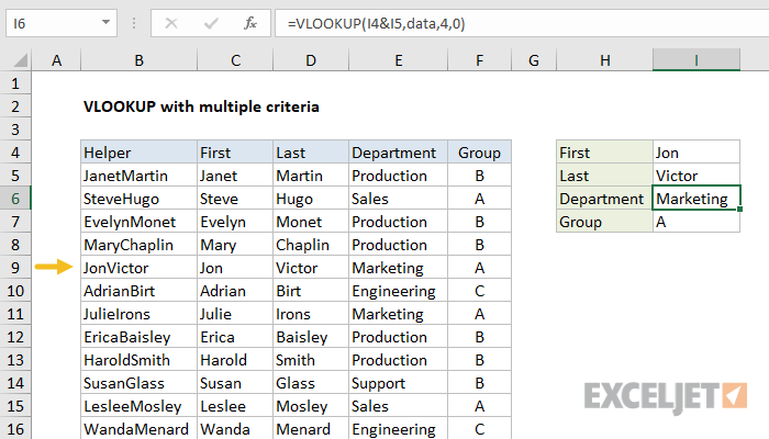
Suppose we have a list of orders and we want to find Quantity of goods (Qty.), based on two criteria – Име клијента (Купац) и Название продукта (Product). The matter is complicated by the fact that each of the buyers ordered several types of goods, as can be seen from the table below:
regular function ВПР will not work in this scenario because it will return the first value it finds that matches the given lookup value. For example, if you want to know the quantity of an item Sweets’ordered by the buyer Џереми Хил, write the following formula:
=VLOOKUP(B1,$A$5:$C$14,3,FALSE)
=ВПР(B1;$A$5:$C$14;3;ЛОЖЬ)
– this formula will return the result 15corresponding to the product јабуке, because it’s the first value that matches.
There is a simple workaround – create an additional column in which to combine all the desired criteria. In our example, these are the columns Име клијента (Купац) и Название продукта (Product). Don’t forget that the merged column must always be the leftmost column in the search range, since it is the left column that the function ВПР looks up when looking for a value.
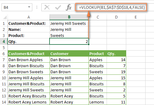
So, you add an auxiliary column to the table and copy the following formula over all its cells: =Б2&Ц2. If you want the string to be more readable, you can separate the combined values with a space: =B2&» «&C2. After that, you can use the following formula:
=VLOOKUP("Jeremy Hill Sweets",$A$7:$D$18,4,FALSE)
=ВПР("Jeremy Hill Sweets";$A$7:$D$18;4;ЛОЖЬ)
or
=VLOOKUP(B1,$A$7:$D$18,4,FALSE)
=ВПР(B1;$A$7:$D$18;4;ЛОЖЬ)
Where is the cell B1 contains the concatenated value of the argument лоокуп_валуе (вредност_потраживања) и 4 – Argument цол_индек_нум (column_number), i.e. the number of the column containing the data to be retrieved.
Example 2: VLOOKUP by two criteria with table being viewed on another sheet
If you need to update the main table (Main table) by adding data from the second table (Lookup table), which is located on another sheet or in another Excel workbook, then you can collect the desired value directly in the formula that you insert into the main table.
As in the previous example, you will need an auxiliary column in the Lookup table with the combined values. This column must be the leftmost column in the search range.
So the formula with ВПР could be like this:
=VLOOKUP(B2&" "&C2,Orders!$A&$2:$D$2,4,FALSE)
=ВПР(B2&" "&C2;Orders!$A&$2:$D$2;4;ЛОЖЬ)
Here, columns B and C contain customer names and product names, respectively, and the link Orders!$A&$2:$D$2 defines a table to look up in another sheet.
To make the formula more readable, you can give the view range a name, and then the formula will look much simpler:
=VLOOKUP(B2&" "&C2,Orders,4,FALSE)
=ВПР(B2&" "&C2;Orders;4;ЛОЖЬ)
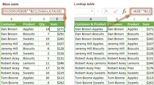
For the formula to work, the values in the leftmost column of the table you are looking at must be combined in exactly the same way as in the search criteria. In the figure above, we combined the values u2bu2band put a space between them, in the same way you need to do in the first argument of the function (BXNUMX& “” & CXNUMX).
Запамтити! функција ВПР limited to 255 characters, it cannot search for a value that is more than 255 characters long. Keep this in mind and make sure that the length of the desired value does not exceed this limit.
I agree that adding an auxiliary column is not the most elegant and not always acceptable solution. You can do the same without the helper column, but that would require a much more complex formula with a combination of functions ИНДЕКС (ИНДЕКС) и УТАКМИЦА (ИЗЛОЖЕНИЈИ).
We extract the 2nd, 3rd, etc. values using VLOOKUP
Ви то већ знате ВПР can return only one matching value, more precisely, the first one found. But what if this value is repeated several times in the viewed array, and you want to extract the 2nd or 3rd of them? What if all values? The problem seems complicated, but the solution exists!
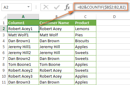
Suppose one column of the table contains the names of the customers (Customer Name), and the other column contains the products (Product) that they bought. Let’s try to find the 2nd, 3rd and 4th items purchased by a given customer.
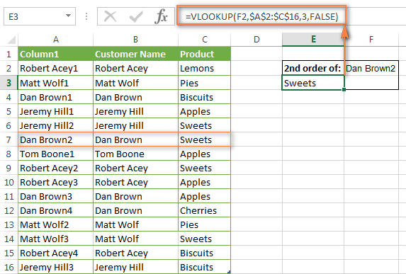
The easiest way is to add an auxiliary column before the column Име клијента and fill it with customer names with the repetition number of each name, for example, John Doe1, John Doe2 etc. We will do the trick with numbering using the function ЦОУНТИФ (COUNTIF), given that the customer names are in column B:
=B2&COUNTIF($B$2:B2,B2)
=B2&СЧЁТЕСЛИ($B$2:B2;B2)
After that you can use the normal function ВПРto find the required order. For example:
- Наћи 2-тх item ordered by the customer Ден Браун:
=VLOOKUP("Dan Brown2",$A$2:$C$16,3,FALSE)=ВПР("Dan Brown2";$A$2:$C$16;3;ЛОЖЬ) - Наћи 3-тх item ordered by the customer Ден Браун:
=VLOOKUP("Dan Brown3",$A$2:$C$16,3,FALSE)=ВПР("Dan Brown3";$A$2:$C$16;3;ЛОЖЬ)
In fact, you can enter a cell reference as the lookup value instead of text, as shown in the following figure:
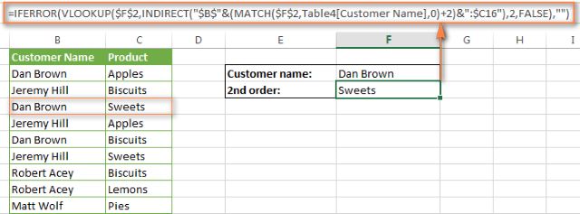
If you are only looking for КСНУМКС-е repetition, you can do it without the auxiliary column by creating a more complex formula:
=IFERROR(VLOOKUP($F$2,INDIRECT("$B$"&(MATCH($F$2,Table4[Customer Name],0)+2)&":$C16"),2,FALSE),"")
=ЕСЛИОШИБКА(ВПР($F$2;ДВССЫЛ("$B$"&(ПОИСКПОЗ($F$2;Table4[Customer Name];0)+2)&":$C16");2;ИСТИНА);"")
У овој формули:
- $F$2 – a cell containing the name of the buyer (it is unchanged, please note – the link is absolute);
- $ B $ – column Име клијента;
- ТаблеКСНУМКС – Your table (this place can also be a regular range);
- $ Ц16 – the end cell of your table or range.
This formula finds only the second matching value. If you need to extract the remaining repetitions, use the previous solution.
If you need a list of all matches – the function ВПР this is not a helper, since it only returns one value at a time – period. But Excel has a function ИНДЕКС (INDEX), which can easily cope with this task. How such a formula will look like, you will learn in the following example.
Retrieve all repetitions of the desired value
Што је горе поменуто ВПР cannot extract all duplicate values from the scanned range. To do this, you need a slightly more complex formula, made up of several Excel functions, such as ИНДЕКС (ИНДЕКС), МАЛА (МАЛА) и РЕД (LINE)
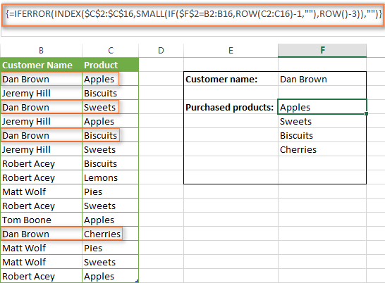
For example, the formula below finds all repetitions of the value from cell F2 in the range B2:B16 and returns the result from the same rows in column C.
{=IFERROR(INDEX($C$2:$C$16,SMALL(IF($F$2=B2:B16,ROW(C2:C16)-1,""),ROW()-3)),"")}
{=ЕСЛИОШИБКА(ИНДЕКС($C$2:$C$16;НАИМЕНЬШИЙ(ЕСЛИ($F$2=B2:B16;СТРОКА(C2:C16)-1;"");СТРОКА()-3));"")}
Enter this array formula into multiple adjacent cells, such as the cells Ф4: Ф8as shown in the figure below. The number of cells must be equal to or greater than the maximum possible number of repetitions of the searched value. Don’t forget to click Цтрл + Схифт + Ентерto enter the array formula correctly.
If you’re interested in understanding how it works, let’s dive into the details of the formula a bit:
Део КСНУМКС:
IF($F$2=B2:B16,ROW(C2:C16)-1,"")
ЕСЛИ($F$2=B2:B16;СТРОКА(C2:C16)-1;"")
$F$2=B2:B16 – compare the value in cell F2 with each of the values in the range B2:B16. If a match is found, then the expression STRING(C2:C16)-1 returns the number of the corresponding line (value -1 allows you to not include the header line). If there are no matches, the function IF (IF) returns an empty string.
Function result IF (IF) there will be such a horizontal array: {1,"",3,"",5,"","","","","","",12,"","",""}
Део КСНУМКС:
ROW()-3
СТРОКА()-3
Овде је функција РЕД (LINE) acts as an additional counter. Since the formula is copied into cells F4:F9, we subtract the number 3 from function result to get value 1 у ћелији F4 (line 4, subtract 3) to get 2 у ћелији F5 (line 5, subtract 3) and so on.
Део КСНУМКС:
SMALL(IF($F$2=B2:B16,ROW(C2:C16)-1,""),ROW()-3))
НАИМЕНЬШИЙ(ЕСЛИ($F$2=B2:B16;СТРОКА(C2:C16)-1;"");СТРОКА()-3))
функција МАЛА (SMALL) returns n-oh the smallest value in the data array. In our case, which position (from the smallest) to return is determined by the function РЕД (LINE) (see Part 2). So, for a cell F4 функција SMALL({array},1) повраћај 1-тх (smallest) array element, i.e. 1. For cell F5 повраћај 2-тх the smallest element in the array, that is 3, Итд
Део КСНУМКС:
INDEX($C$2:$C$16,SMALL(IF($F$2=B2:B16,ROW(C2:C16)-1,""),ROW()-3))
ИНДЕКС($C$2:$C$16;НАИМЕНЬШИЙ(ЕСЛИ($F$2=B2:B16;СТРОКА(C2:C16)-1;"");СТРОКА()-3))
функција ИНДЕКС (INDEX) simply returns the value of a specific cell in an array Ц2: Ц16. For cell F4 функција INDEX($C$2:$C$16) ће се вратити јабукеза F5 функција INDEX($C$2:$C$16) ће се вратити Sweets’ и тако даље.
Део КСНУМКС:
IFERROR()
ЕСЛИОШИБКА()
Finally, we put the formula inside the function ИФЕРРОР (IFERROR), because you are unlikely to be pleased with the error message #АТ (#N/A) if the number of cells into which the formula is copied is less than the number of duplicate values in the range being viewed.
XNUMXD search by known row and column
Performing a XNUMXD search in Excel involves searching for a value by a known row and column number. In other words, you are extracting the cell value at the intersection of a particular row and column.
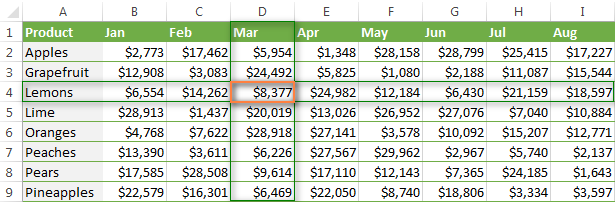
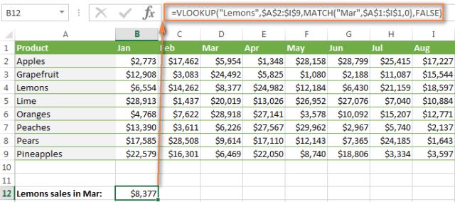
So, let’s turn to our table and write a formula with a function ВПР, which will find information about the cost of lemons sold in March.
There are several ways to perform a XNUMXD search. Check out the options and choose the one that suits you best.
VLOOKUP and MATCH functions
You can use a bunch of functions ВПР (ВЛООКУП) и ИЗЛОЖЕНИЈИ (MATCH) to find the value at the intersection of the fields Название продукта (string) and месец (column) of the array in question:
=VLOOKUP("Lemons",$A$2:$I$9,MATCH("Mar",$A$1:$I$1,0),FALSE)
=ВПР("Lemons";$A$2:$I$9;ПОИСКПОЗ("Mar";$A$1:$I$1;0);ЛОЖЬ)
The formula above is a regular function ВПР, which looks for an exact match of the value “Lemons” in cells A2 through A9. But since you don’t know which column the March sales are in, you won’t be able to set the column number for the third function argument. ВПР. Instead, the function is used ИЗЛОЖЕНИЈИto define this column.
MATCH("Mar",$A$1:$I$1,0)
ПОИСКПОЗ("Mar";$A$1:$I$1;0)
Translated into human language, this formula means:
- We are looking for the characters “Mar” – argument лоокуп_валуе (lookup_value);
- Looking in cells from A1 to I1 – argument лоокуп_арраи (lookup_array);
- Returning exact match – argument матцх_типе (match_type).
Коришћење 0 in the third argument, you say functions ИЗЛОЖЕНИЈИ look for the first value that exactly matches the value you are looking for. This is equivalent to the value ЛАЖ (FALSE) for the fourth argument ВПР.
This is how you can create a two-way search formula in Excel, also known as two-dimensional search or bidirectional search.
Функција СУМПРОДУЦТ
функција СУМПРОДУЦТ (SUMPRODUCT) returns the sum of the products of the selected arrays:
=SUMPRODUCT(($A$2:$A$9="Lemons")*($A$1:$I$1="Mar"),$A$2:$I$9)
=СУММПРОИЗВ(($A$2:$A$9="Lemons")*($A$1:$I$1="Mar");$A$2:$I$9)
INDEX and MATCH functions
In the next article I will explain these functions in detail, so for now you can just copy this formula:
=INDEX($A$2:$I$9,MATCH("Lemons",$A$2:$A$9,0),MATCH("Mar",$A$1:$I$1,0))
=ИНДЕКС($A$2:$I$9;ПОИСКПОЗ("Lemons";$A$2:$A$9;0);ПОИСКПОЗ("Mar";$A$1:$I$1;0))
Named ranges and the intersection operator
If you’re not into all those complex Excel formulas, you might like this visual and memorable way:
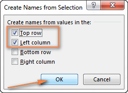
- Select the table, open the tab формула (Формуле) и кликните Креирајте из селекције (Create from selection).
- Означите поља Top row (on the line above) and Лева колона (in the column on the left). Microsoft Excel will assign names to the ranges from the values in the top row and left column of your spreadsheet. Now you can search using these names directly without creating formulas.

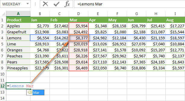
- In any empty cell, write =row_name column_name, for example like this:
=Lemons Mar
… or vice versa:
=Mar Lemons
Remember that the row and column names must be separated by a space, which in this case works like the intersection operator.
When you enter a name, Microsoft Excel will show a tooltip with a list of matching names, just like when you enter a formula.
- Press унети and check the result
In general, whichever of the above methods you choose, the result of a two-dimensional search will be the same:
Using multiple VLOOKUPs in one formula
It happens that the main table and the lookup table do not have a single column in common, and this prevents you from using the usual function ВПР. However, there is another table that does not contain the information we are interested in, but has a common column with the main table and the lookup table.
Let’s take a look at the following example. We have a Main table with a column SKU (new), where you want to add a column with the corresponding prices from another table. In addition, we have 2 lookup tables. The first one (Lookup table 1) contains updated numbers SKU (new) and product names, and the second (Lookup table 2) – product names and old numbers SKU (old).
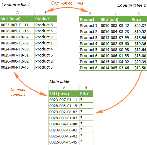
To add prices from the second lookup table to the main table, you must perform an action known as double ВПР или угнежђене ВПР.
- Напишите функцију ВПР, which finds the product name in the table Lookup table 1коришћење Шифра, as the desired value:
=VLOOKUP(A2,New_SKU,2,FALSE)=ВПР(A2;New_SKU;2;ЛОЖЬ)Овде New_SKU – named range $A:$B у табели Lookup table 1, 2 – this is column B, which contains the names of the goods (see the picture above)
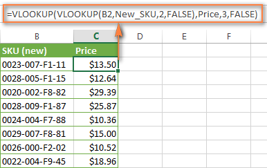
- Write a formula to insert prices from a table Lookup table 2 based on well-known product names. To do this, paste the formula you created earlier as the lookup value for the new function ВПР:
=VLOOKUP(VLOOKUP(A2,New_SKU,2,FALSE),Price,3,FALSE)=ВПР(ВПР(A2;New_SKU;2;ЛОЖЬ);Price;3;ЛОЖЬ)Овде Cena – named range $А:$Ц у табели Lookup table 2, 3 is column C containing prices.
The figure below shows the result returned by the formula we created:
Dynamic substitution of data from different tables using VLOOKUP and INDIRECT
First, let’s clarify what we mean by the expression “Dynamic substitution of data from different tables” to make sure we understand each other correctly.
There are situations when there are several sheets with data of the same format, and it is necessary to extract the necessary information from a certain sheet, depending on the value that is entered in a given cell. I think it’s easier to explain this with an example.
Imagine that you have sales reports for several regions with the same products and in the same format. You want to find sales figures for a specific region:
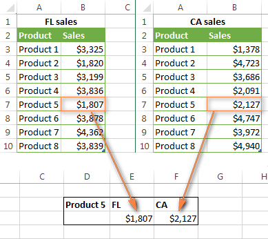
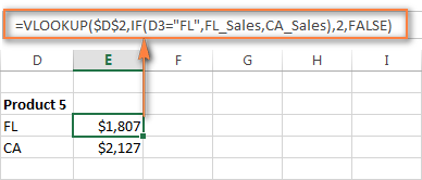
If you have only two such reports, then you can use a disgracefully simple formula with functions ВПР и IF (IF) to select the desired report to search:
=VLOOKUP($D$2,IF($D3="FL",FL_Sales,CA_Sales),2,FALSE)
=ВПР($D$2;ЕСЛИ($D3="FL";FL_Sales;CA_Sales);2;ЛОЖЬ)
Где:
- $ Д $ 2 is a cell containing the name of the product. Note that we use absolute references here to avoid changing the lookup value when copying the formula to other cells.
- $D3 is a cell with the name of the region. We are using an absolute column reference and a relative row reference because we plan to copy the formula to other cells in the same column.
- FL_Sales и CA_Sales – the names of the tables (or named ranges) that contain the corresponding sales reports. You can, of course, use the usual sheet names and cell range references, for example ‘FL Sheet’!$A$3:$B$10, but named ranges are much more convenient.
However, when there are many such tables, the function IF is not the best solution. Instead, you can use the function ИНДИРЕКТАН (INDIRECT) to return the desired search range.
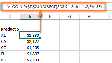
As you probably know, the function ИНДИРЕКТАН is used to return a link given by a text string, which is exactly what we need now. So, boldly replace in the above formula the expression with the function IF to link with function ИНДИРЕКТАН. Here is a combination ВПР и ИНДИРЕКТАН works great with:
=VLOOKUP($D$2,INDIRECT($D3&"_Sales"),2,FALSE)
=ВПР($D$2;ДВССЫЛ($D3&"_Sales");2;ЛОЖЬ)
Где:
- $ Д $ 2 – this is a cell with the name of the product, it is unchanged due to the absolute link.
- $D3 is the cell containing the first part of the region name. In our example, this FL.
- _Sales – the common part of the name of all named ranges or tables. When combined with the value in cell D3, it forms the fully qualified name of the required range. Below are some details for those who are new to the function ИНДИРЕКТАН.
How INDIRECT and VLOOKUP work
First, let me remind you the syntax of the function ИНДИРЕКТАН (ИНДИРЕКТАН):
INDIRECT(ref_text,[a1])
ДВССЫЛ(ссылка_на_текст;[a1])
The first argument can be a cell reference (A1 or R1C1 style), a range name, or a text string. The second argument determines what style of link is contained in the first argument:
- A1ако је аргумент ТРУЕ ЦОДЕ (TRUE) or not specified;
- РКСНУМКСЦКСНУМКС, Ако FAS E (ФАЛСЕ).
In our case, the link has the style A1, so you can leave out the second argument and focus on the first.
So let’s get back to our sales reports. If you remember, then each report is a separate table located on a separate sheet. For the formula to work correctly, you must name your tables (or ranges), and all names must have a common part. For example, like this: CA_Sales, FL_Sales, TX_Sales and so on. As you can see, “_Sales” is present in all the names.
функција ИНДИРЕКТАН connects the value in column D and the text string “_Sales”, thereby telling ВПР in which table to search. If cell D3 contains the value “FL”, the formula will search the table FL_Sales, if “CA” – in the table CA_Sales и тако даље.
The result of the functions ВПР и ИНДИРЕКТАН биће следеће:
If the data is located in different Excel books, then you need to add the name of the book before the named range, for example:
=VLOOKUP($D$2,INDIRECT($D3&"Workbook1!_Sales"),2,FALSE)
=ВПР($D$2;ДВССЫЛ($D3&"Workbook1!_Sales");2;ЛОЖЬ)
If the function ИНДИРЕКТАН refers to another workbook, that workbook must be open. If it is closed, the function will report an error. #РЕФ! (#ССИЛ!).