


Садржај
Јуче на маратону 30 Екцел функција за 30 дана we found the elements of the array using the function УТАКМИЦА (SEARCH) and found that it works great in a team with other features such as ВЛООКУП (ВЛООКУП) и ИНДЕКС (ИНДЕКС).
On the 20th day of our marathon, we will devote the study of the function АДРЕСА (ADDRESS). It returns the cell address in text format using the row and column number. Do we need this address? Can the same be done with other functions?
Let’s take a look at the details of the function АДРЕСА (ADDRESS) and study examples of working with it. If you have additional information or examples, please share them in the comments.
Function 20: ADDRESS
функција АДРЕСА (ADDRESS) returns a cell reference as text based on the row and column number. It can return an absolute or relative link-style address. A1 or РКСНУМКСЦКСНУМКС. In addition, the sheet name can be included in the result.
How can the ADDRESS function be used?
функција АДРЕСА (ADDRESS) can return the address of a cell, or work in conjunction with other functions to:
- Get cell address given row and column number.
- Find cell value by knowing row and column number.
- Return the address of the cell with the largest value.
Syntax ADDRESS (ADDRESS)
функција АДРЕСА (ADDRESS) has the following syntax:
ADDRESS(row_num,column_num,[abs_num],[a1],[sheet_text])
АДРЕС(номер_строки;номер_столбца;[тип_ссылки];[а1];[имя_листа])
- abs_num (link_type) – if equal 1 or not specified at all, the function will return the absolute address ($A$1). To get the relative address (A1), use the value 4. Друге опције: 2=A$1, 3=$A1.
- a1 – if TRUE (TRUE) or not specified at all, the function returns a reference in the style A1, if FALSE (FALSE), then in style РКСНУМКСЦКСНУМКС.
- Лист_text (sheet_name) – the name of the sheet can be specified if you want to see it in the result returned by the function.
Traps ADDRESS
функција АДРЕСА (ADDRESS) returns only the address of the cell as a text string. If you need the value of a cell, use it as a function argument ИНДИРЕКТАН (INDIRECT) or use one of the alternative formulas shown in Example 2.
Example 1: Get cell address by row and column number
Коришћење функција АДРЕСА (ADDRESS) You can get the cell address as text using the row and column number. If you enter only these two arguments, the result will be an absolute address written in link style A1.
=ADDRESS($C$2,$C$3)
=АДРЕС($C$2;$C$3)
Absolute or relative
If you do not specify an argument value abs_num (reference_type) in a formula, the result is an absolute reference.
To see the address as a relative link, you can substitute as an argument abs_num (reference_type) value 4.
=ADDRESS($C$2,$C$3,4)
=АДРЕС($C$2;$C$3;4)
A1 or R1C1
To style links РКСНУМКСЦКСНУМКС, instead of the default style A1, You must specify FALSE for the argument a1.
=ADDRESS($C$2,$C$3,1,FALSE)
=АДРЕС($C$2;$C$3;1;ЛОЖЬ)
Назив листа
The last argument is the name of the sheet. If you need this name in the result, specify it as an argument sheet_text (sheet_name).
=ADDRESS($C$2,$C$3,1,TRUE,"Ex02")
=АДРЕС($C$2;$C$3;1;ИСТИНА;"Ex02")
Example 2: Find cell value using row and column number
функција АДРЕСА (ADDRESS) returns the address of the cell as text, not as a valid link. If you need to get the value of a cell, you can use the result returned by the function АДРЕСА (ADDRESS), as an argument for ИНДИРЕКТАН (INDIRECT). We will study the function ИНДИРЕКТАН (INDIRECT) later in the marathon 30 Екцел функција за 30 дана.
=INDIRECT(ADDRESS(C2,C3))
=ДВССЫЛ(АДРЕС(C2;C3))
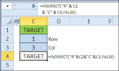
функција ИНДИРЕКТАН (INDIRECT) can work without the function АДРЕСА (ADDRESS). Here’s how you can, using the concatenation operator “&“, blind the desired address in the style РКСНУМКСЦКСНУМКС and as a result get the value of the cell:
=INDIRECT("R"&C2&"C"&C3,FALSE)
=ДВССЫЛ("R"&C2&"C"&C3;ЛОЖЬ)
функција ИНДЕКС (INDEX) can also return the value of a cell if a row and column number is specified:
=INDEX(1:5000,C2,C3)
=ИНДЕКС(1:5000;C2;C3)
1:5000 are the first 5000 rows of an Excel sheet.
Example 3: Return the address of the cell with the maximum value
In this example, we will find the cell with the maximum value and use the function АДРЕСА (ADDRESS) to get her address.
функција МАКС (MAX) finds the maximum number in column C.
=MAX(C3:C8)
=МАКС(C3:C8)
Next comes the function АДРЕСА (ADDRESS) combined with УТАКМИЦА (MATCH), which finds the line number, and КОЛОНА (COLUMN), which specifies the column number.
=ADDRESS(MATCH(F3,C:C,0),COLUMN(C2))
=АДРЕС(ПОИСКПОЗ(F3;C:C;0);СТОЛБЕЦ(C2))