Уметање и подешавање слике у Екцел-у

Sometimes, to perform certain tasks in Excel, you need to insert some kind of picture or photo into the table. Let’s see how exactly this can be done in the program.

Белешка: before proceeding directly to the procedure for inserting a picture into Excel, you need to have it at hand – on the computer’s hard drive or USB drive that is connected to the PC.

Уметање слике на лист

To begin with, we carry out preparatory work, namely, open the desired document and go to the required sheet. We proceed according to the following plan:

1. We get up in the cell where we plan to insert the picture. Switch to tab „Убаци“где кликнемо на дугме “Илустрације”. In the drop-down list, select the item “Drawings”.
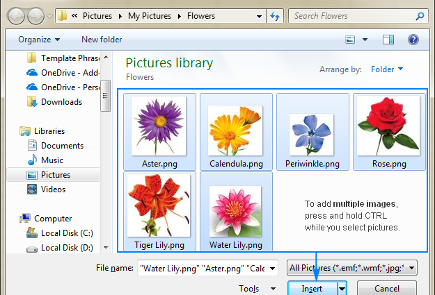
2. A window will appear on the screen in which you need to select the desired image. To do this, first go to the folder containing the required file (by default, the folder “Слике”), then click on it and press the button „Отворено“ (or you can just double-click on the file).
3. As a result, the selected picture will be inserted on the sheet of the book. However, as you can see, it just placed on top of the cells and has nothing to do with them. So let’s move on to the next steps.

Подешавање слике

Now we need to adjust the inserted image by giving it the desired dimensions.

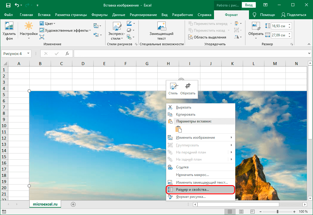
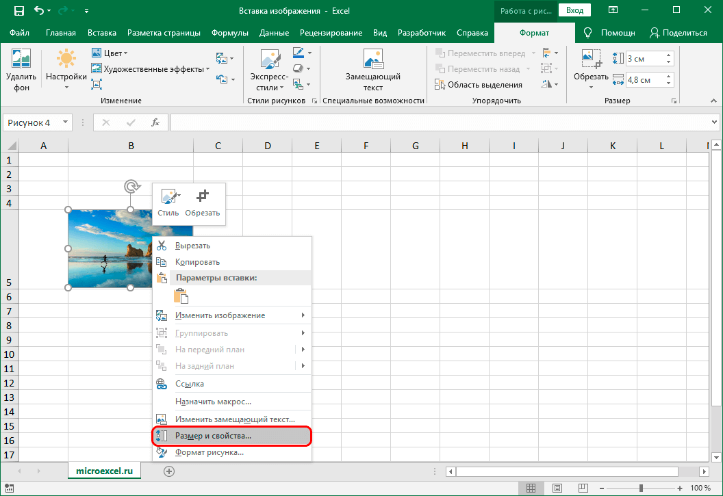
1. Click on the picture with the right mouse button. In the dropdown list, select “Size and Properties”.
2. A picture format window will appear, where we can fine-tune its parameters:
   • dimensions (height and width);
   • angle of rotation;
   • height and width as a percentage;
   • keeping proportions, etc..
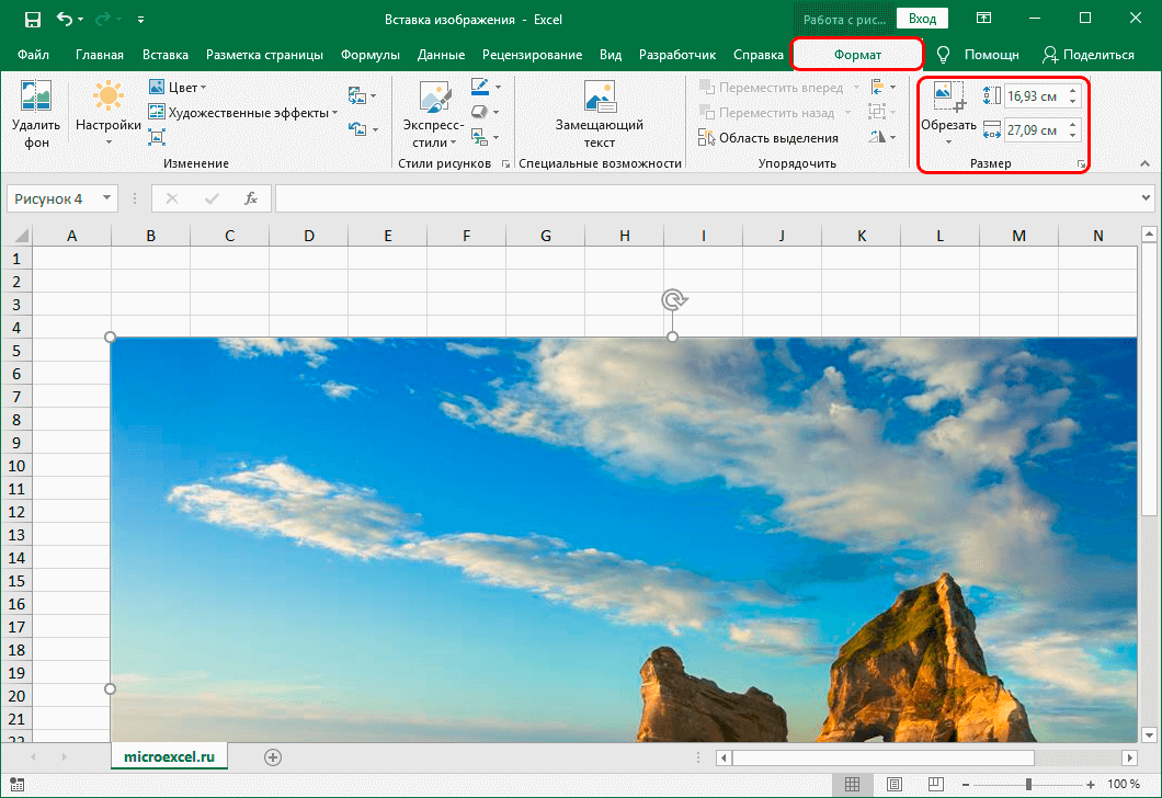
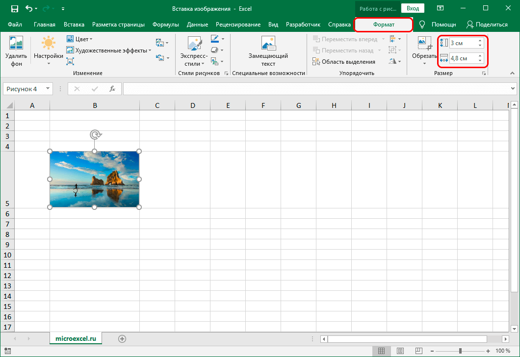
3. However, in most cases, instead of going to the picture format window, the settings that can be made in the tab "Формат" (in this case, the drawing itself should be selected).
4. Let’s say we need to adjust the size of the image so that it does not go beyond the boundaries of the selected cell. You can do this in different ways:
   • идите на Подешавања “Dimensions and Properties” through the context menu of the picture and adjust the size in the window that appears.
   • set the dimensions using the appropriate tools in the tab "Формат" on the program ribbon.
   • holding the left mouse button, drag the lower right corner of the picture diagonally upwards.

Attaching an image to a cell

So, we inserted a picture on an Excel sheet and adjusted its size, which allowed us to fit it into the borders of the selected cell. Now you need to attach a picture to this cell. This is done so that in cases where a change in the structure of the table leads to a change in the original location of the cell, the picture moves with it. You can implement this in the following way:

1. We insert an image and adjust its size to fit the cell borders, as described above.
2. Click on the image and select from the list “Size and Properties”.
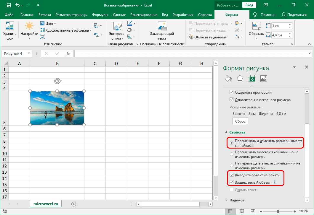
3. Before us, the already familiar picture format window will appear. After making sure that the dimensions correspond to the desired values, and also that there are checkboxes “Keep proportions” и “Relative to the original size”, go к "Својства".
4. In the properties of the picture, put the checkboxes in front of the items “Protected object” и “Print object”. Also, select the option “Move and resize with cells”.

Protecting a cell with an image from changes

This measure, as the name of the header implies, is needed in order to protect the cell containing the picture from being changed and deleted. Here is what you need to do for this:

1. Select the entire sheet, for which we first remove the selection from the image by clicking on any other cell, and then press the key combination Цтрл + А. Then we call the context menu of the cells by right-clicking anywhere in the selected area and select the item „Формат ћелије“.
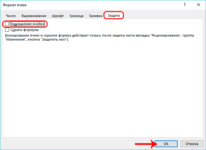
2. In the formatting window, switch to the tab "Заштита", where we uncheck the box opposite the item "Заштићена ћелија" и кликните на дугме OK.
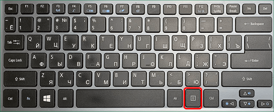
3. Now click on the cell where the picture was inserted. After that, also through the context menu, go to its format, then go to the tab "Заштита". Check the box next to the option "Заштићена ћелија" и кликните на дугме OK.Белешка: if a picture inserted into a cell completely overlaps it, then clicking on it with the mouse buttons will call up the properties and settings of the picture itself. Therefore, in order to go to a cell with an image (select it), it is best to click on any other cell next to it, and then, using the navigation keys on the keyboard (up, down, right, left), go to the required one. Also, to call the context menu, you can use a special key on the keyboard, which is located to the left of Цтрл.
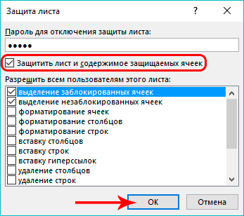
4. Пребаците се на картицу “Преглед”where click on the button „Заштитни лист“ (when the window dimensions are compressed, you must first click the button "Заштита", after which the desired item will appear in the drop-down list).
5. A small window will appear where we can set a password to protect the sheet and a list of actions that users can perform. Click when ready OK.
6. In the next window, confirm the entered password and click У РЕДУ.
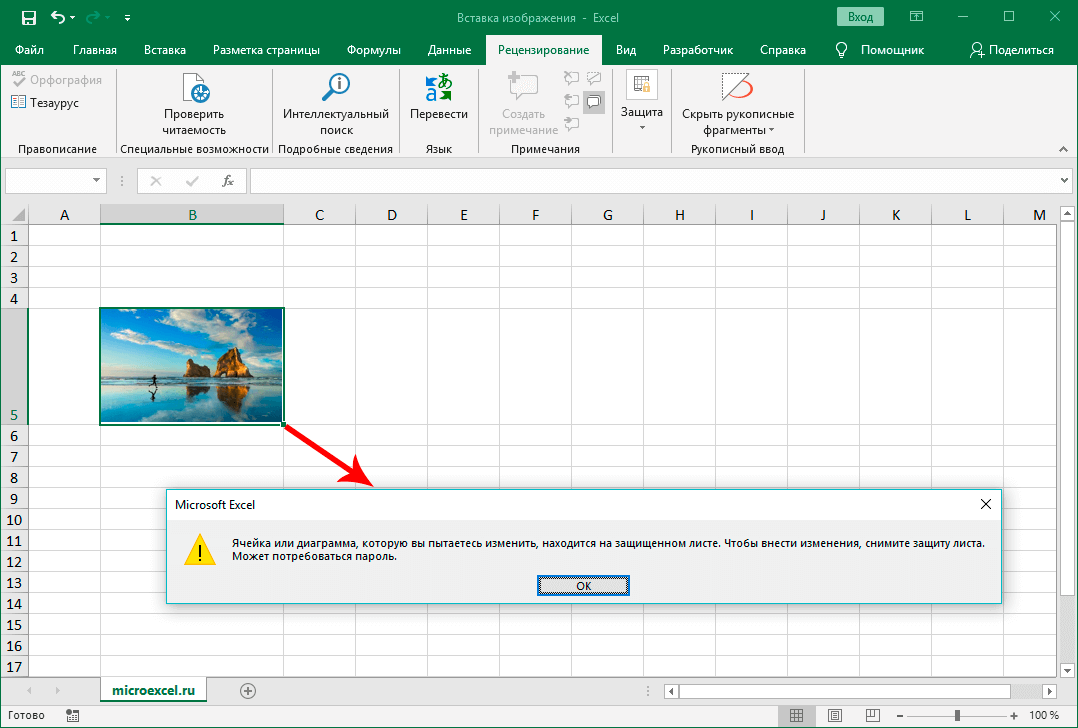
7. As a result of the performed actions, the cell in which the picture is located will be protected from any changes, incl. removal.At the same time, the remaining cells of the sheet remain editable, and the degree of freedom of action in relation to them depends on which items we selected when the sheet protection was turned on.

Inserting an image into a cell comment

In addition to inserting a picture into a table cell, you can add it to a note. How this is done is described below:

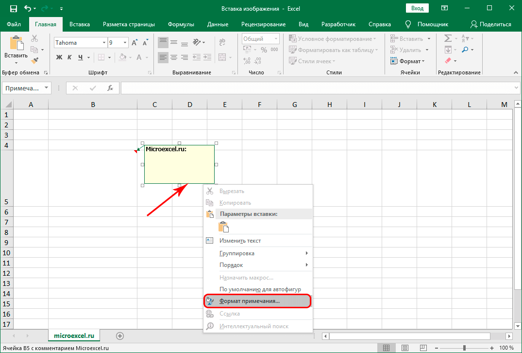
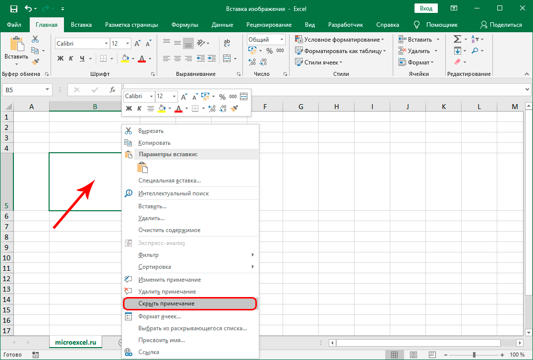
1. Right-click on the cell where you want to insert the image. In the drop-down list, select the command “Insert note”.
2. A small area for entering a note will appear. Hover the cursor over the border of the note area, right-click on it and in the list that opens, click on the item “Note Format”.
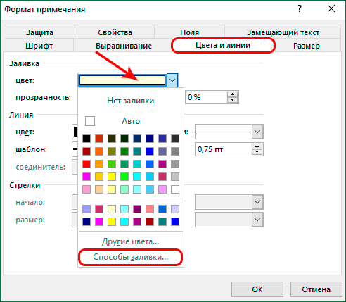
3. The note settings window will appear on the screen. Switch to tab “Colors and Lines”. In the fill options, click on the current color. A list will open in which we select the item „Методе попуњавања“.
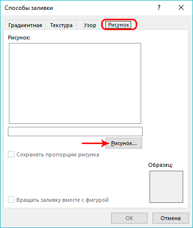
4. In the fill methods window, switch to the tab „Слика“, where we press the button with the same name.
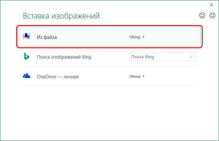
5. An image insertion window will appear, in which we select the option “From file”.
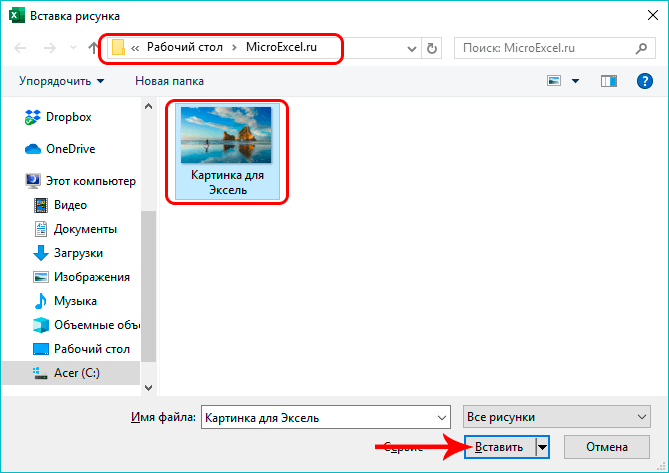
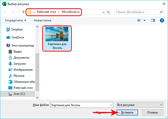
6. After that, a picture selection window will open, which we already encountered at the beginning of our article. Go to the folder containing the file with the desired image, then press the button „Убаци“.
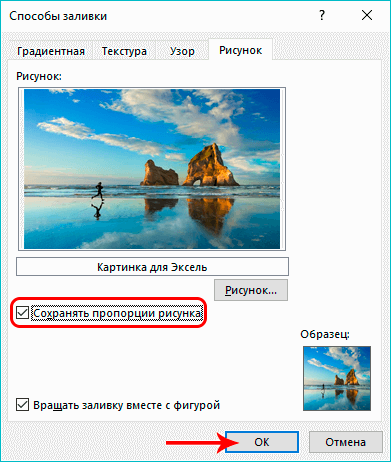
7. The program will return us to the previous window for selecting fill methods with the selected pattern. Check the box for the option “Keep the proportions of the picture”, а затим кликните OK.
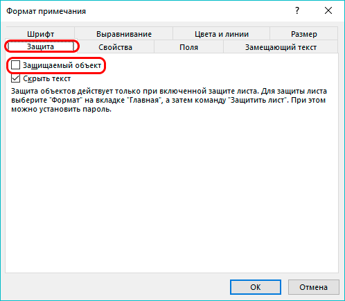
8. After that, we will find ourselves in the main note format window, where we switch to the tab "Заштита". Here, uncheck the box next to the item “Protected Object”.
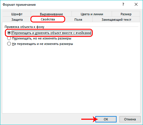
9. Next, go to the tab "Својства". Choose an option “Move and change object along with cells”. All settings are made, so you can press the button OK.
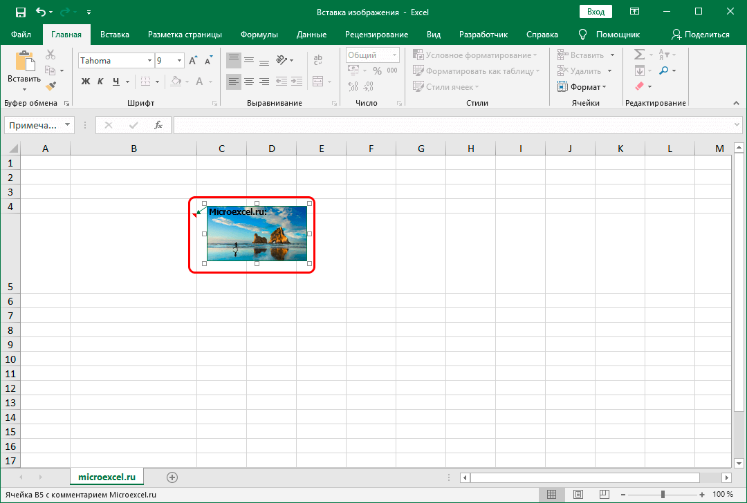
10. As a result of the actions performed, we managed not only to insert a picture as a note to the cell, but also to attach it to the cell.
11. If desired, the note can be hidden. In this case, it will only be displayed when you hover over the cell. To do this, right-click on the cell with a note and select the item in the context menu “Hide note”.If necessary, the note is included back in the same way.

Insert image in developer mode

Excel also provides the ability to insert a picture into a cell through the so-called Режим програмера. But first you need to activate it, since it is disabled by default.

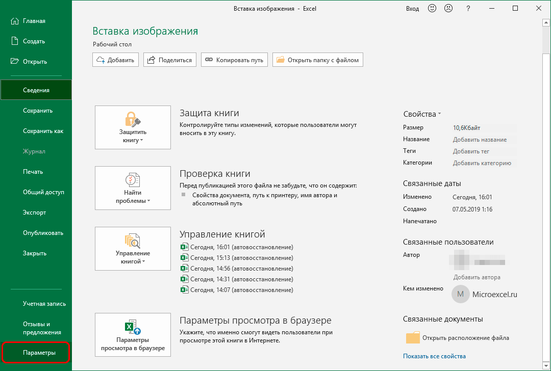
1. Идите на мени „Датотека“, where we click on the item „Параметри“.
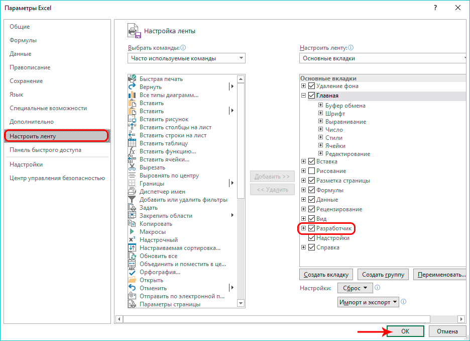
2. A window of parameters will open, where in the list on the left click on the section „Прилагоди траку“. After that, in the right part of the window in the ribbon settings, we find the line „Програмер“, check the box next to it and click OK.
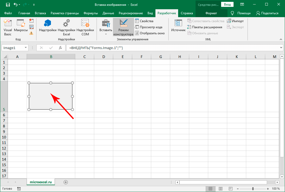
3. We stand in the cell where we want to insert the image, and then go to the tab „Програмер“. In the tools section “Controls” find the button „Убаци“ and click on it. In the list that opens, click on the icon “Image” у групи “Active controls”.
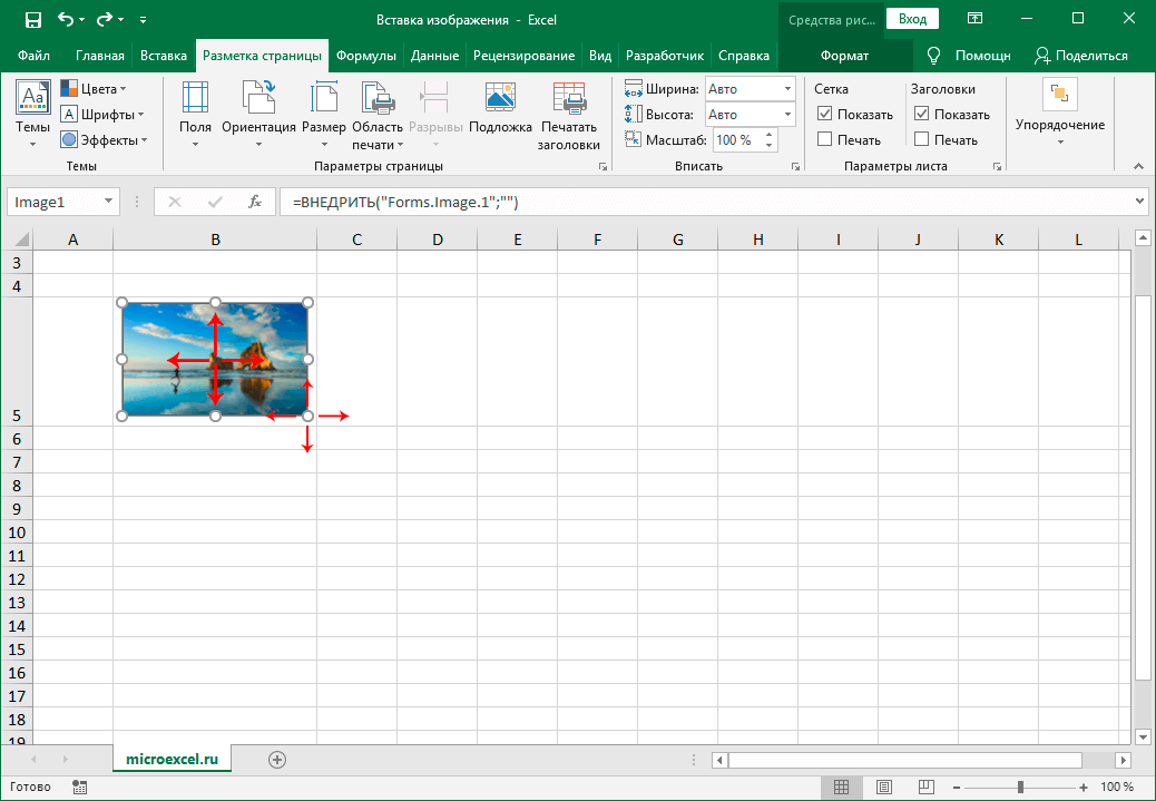
4. The cursor will change to a cross. With the left mouse button pressed, select the area for the future image. If necessary, the dimensions of this area can then be adjusted or the location of the resulting rectangle (square) can be changed to fit it inside the cell.
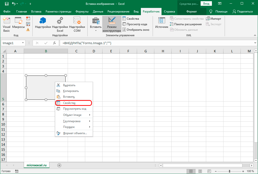
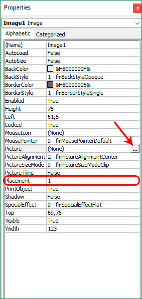
5. Right-click on the resulting figure. In the drop-down list of commands, select "Својства".
6. We will see a window with the properties of the element:
   • in parameter value "Постављање" indicate the number "КСНУМКС" (initial value – "КСНУМКС").
   • in the field for entering a value opposite the parameter „Слика“ click on the button with three dots.
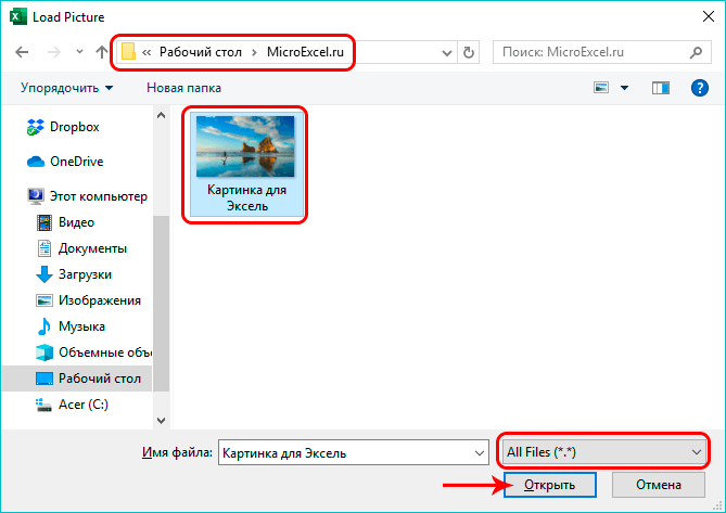
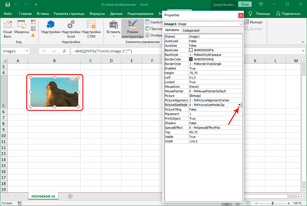
7. An image upload window will appear. We select the desired file here and open it by clicking the appropriate button (it is recommended to select the file type “All Files”, because otherwise some of the extensions will not be visible in this window).
8. As you can see, the picture is inserted on the sheet, however, only a part of it is displayed, so size adjustment is required. To do this, click on the icon in the form of a small triangle down in the parameter value field “PictureSizeMode”.
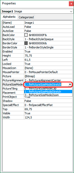
9. In the drop-down list, select the option with the number “1” at the beginning.
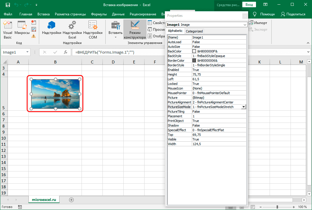
10. Now the whole image fits inside the rectangular area, so the settings can be closed.
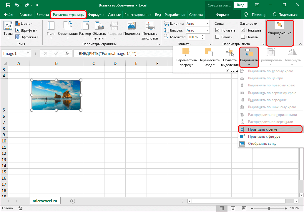
11. It remains only to bind the image to the cell. To do this, go to the tab "Распоред на страници", where we press the button “Ordering”. In the drop-down list, select the item "Поравнајте", онда - “Snap to Grid”.
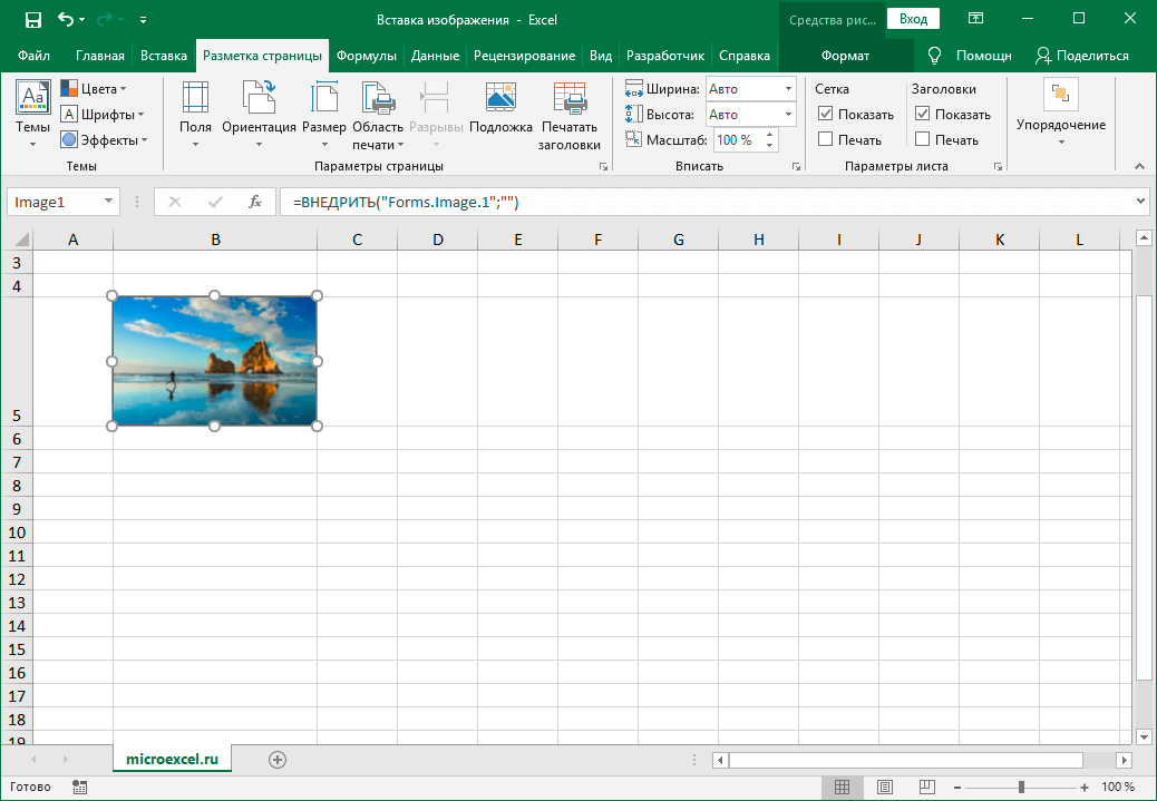
12. Done, the picture is attached to the selected cell. In addition, now its borders will “stick” to the borders of the cell if we move the image or resize it.
13. This will allow you to accurately fit the picture into the cell without much effort.

Zakljucak

Thus, there are several ways in which you can insert an image into a cell on an Excel sheet. The easiest method is to use the tools in the Insert tab, so it’s no surprise that this is the most popular method among users. In addition, it is possible to insert images as cell notes or add pictures to a sheet using a special Developer Mode.