


Who is too lazy or does not have time to read – watch the video. Details and nuances are in the text below.
Формулисање проблема
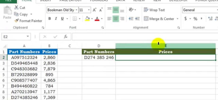
So, we have two tables – order table и Ценовник:
The task is to substitute prices from the price list into the table of orders automatically, focusing on the name of the product so that later you can calculate the cost.
Решење
In the Excel function set, under the category Референце и низови (Lookup and reference) there is a function ВПР (ВЛООКУП).This function looks for a given value (in our example, this is the word “Apples”) in the leftmost column of the specified table (price list) moving from top to bottom and, having found it, displays the contents of the adjacent cell (23 rubles) .Schematically, the operation of this function can be represented So:
For ease of further use of the function, do one thing at once – give the range of cells in the price list your own name. To do this, select all the cells of the price list except for the “header” (G3: H19), select from the menu Убаци – Име – Додели (Уметнути — Име — Дефинисати) или притисните ЦТРЛ + ФКСНУМКС and enter any name (no spaces) like Cena… Now, in the future, you can use this name to link to the price list.
Сада користимо функцију ВПР… Select the cell where it will be entered (D3) and open the tab Formulas – Function Insertion (Формуле — Убаци функцију)… У категорији Референце и низови (Потрага и референца) find the function ВПР (ВЛООКУП) и притисните OK… A window for entering arguments for the function will appear:

We fill them in turn:
- Жељена вредност (Lookup Value) – the name of the product that the function should find in the leftmost column of the price list. In our case, the word “Apples” from cell B3.
- Табела (Table Array) – a table from which the desired values uXNUMXbuXNUMXbare taken, that is, our price list. For reference, we use our own name “Price” given earlier. If you didn’t give a name, you can just select the table, but don’t forget to press the button F4to pin the link with dollar signs, because otherwise, it will slide down when copying our formula down to the rest of the cells in column D3:D30.
- Колона_број (Column index number) – serial number (not a letter!) Of the column in the price list from which we will take price values. The first column of the price list with the names is numbered 1, therefore we need the price from the column numbered 2.
- interval_lookup (Range Lookup) – only two values can be entered in this field: FALSE or TRUE:
- If a value is entered 0 or ЛЕЖАЊЕ (НЕТАЧНО), then in fact this means that only search is allowed Тачан меч, i.e. if the function does not find the non-standard item specified in the order table in the price list (if “Coconut” is entered, for example), it will generate the #N/A (no data) error.
- If a value is entered 1 or ТАЧНО (ИСТИНИТО), then this means that you allow the search not for the exact, but approximate match, i.e. in the case of “coconut”, the function will try to find a product with a name that is as close as possible to “coconut” and return the price for this name. In most cases, such an approximate substitution can play a trick on the user by substituting the value of the wrong product that was actually there! So for most real business problems, approximate search is best not to allow. The exception is when we are looking for numbers and not text – for example, when calculating Step Discounts.
Everything! It remains to press OK and copy the entered function to the entire column.
# N / A errors and their suppression
функција ВПР (ВЛООКУП) returns #N/A error (#Н/А) ако:
- Exact search enabled (argument Interval view = 0) and the desired name is not in Табела.
- Coarse search included (Interval view = 1), али Табела, in which the search is taking place is not sorted in ascending order of names.
- The format of the cell where the required value of the name comes from (for example, B3 in our case) and the format of the cells of the first column (F3: F19) of the table are different (for example, numeric and text). This case is especially typical when using numeric codes (account numbers, identifiers, dates, etc.) instead of text names. In this case, you can use the functions Ч и ТЕКСТ to convert data formats. It will look something like this:
=VLOOKUP(TEXT(B3),price,0)
Више о овоме можете прочитати овде.
- The function cannot find the required value because the code contains spaces or invisible non-printable characters (line breaks, etc.). In this case, you can use text functions ТРИМ (ТРИМ) и ПРИНТ(ЧИСТ) to remove them:
=VLOOKUP(TRIMSPACES(CLEAN(B3)),price,0)
=VLOOKUP(TRIM(CLEAN(B3));price;0)
To suppress the error message # Н / А (#Н/А) in cases where the function cannot find an exact match, you can use the function ИФЕРРОР (ИФЕРРОР)… So, for example, this construction intercepts any errors generated by the VLOOKUP and replaces them with zeros:
= IFERROR (VLOOKUP (B3, price, 2, 0), 0)
= IFERROR (VLOOKUP (B3; price; 2; 0); 0)
PS
If you need to extract not one value, but the entire set at once (if there are several different ones), then you will have to shamanize with the array formula. or use the new XLOOKUP feature from Office 365.
- An improved version of the VLOOKUP function (VLOOKUP 2).
- Quick calculation of step (range) discounts using the VLOOKUP function.
- How to make a “left VLOOKUP” using the INDEX and MATCH functions
- How to use the VLOOKUP function to fill in the forms with data from the list
- How to pull out not the first, but all the values from the table at once
- ВЛООКУП2 и ВЛООКУП3 функције из ПЛЕКС додатка